Return per unit of risk: how to evaluate a portfolio properly

Investors often reduce performance evaluation to a single question: how much money did I make? Of course, that is the goal. Although a proper assessment requires more than one number: beyond return, we need to consider costs, currency, inflation, the investment horizon, risk, benchmark performance, and other factors. The same headline return can conceal very different financial outcomes.

Consider two portfolios, each starting with 100 million rubles: after one year, both are worth 125 million (a 25% return). Yet their dynamics differ.

The first portfolio reached 120 million rubles, then fell to 105 and recovered to 125; its maximum drawdown was 12.5%. The second also reached 120, but fell to 90 million and only then returned to 125; its drawdown was 25%.

The final return is the same, but the investor’s experience is very different: the return-to-risk ratio for the first portfolio equals two (25 / 12.5), while for the second it equals one (25 / 25). In the first case, the same 25% return came at half the drawdown.

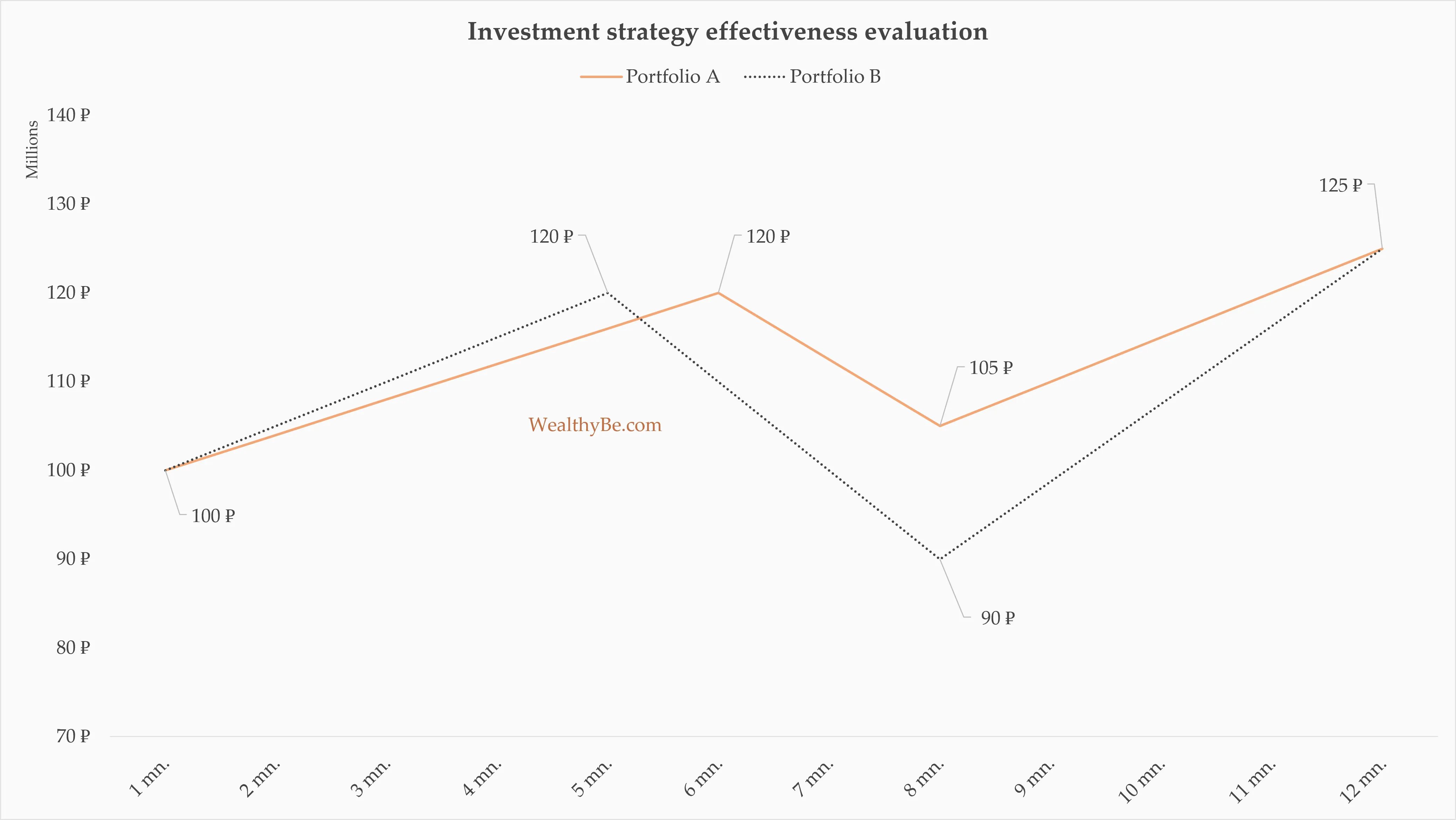
The recovery period matters, too: the first portfolio’s drawdown lasted 4 months, not 6 as in the second case.

Return without risk tells us only where the portfolio ended up, not what it took to get there. But when capital supports personal goals, family well-being, and long-term plans, this path is critically important.

Below, we will look at the metrics that help evaluate investment results more fully: different types of return and risk, alpha and beta, Sharpe and Sortino ratios. I am not trying to turn you into a mathematician or a risk manager, but reducing the evaluation of investment decisions exclusively to return is also wrong.

Which return are we talking about?

Not all returns are created equal. Boring? Perhaps. But unavoidable. In practice, confusion arises constantly.

One investor says they made “10%,” another says “30%,” and a third claims to have doubled their money. From academical point of view, this is usually the simplest metric – holding period return (HPR). Although the period is often missing. Yet 10% earned over a year is clearly better than 30% earned over four. HPR works only as a rough “before and after” measure, but it is insufficient for comparing strategies, funds, or portfolios with one another.

Arithmetic average return can be useful for estimating expected returns over the next period (for example, a month, quarter, or year), but it is not suitable for analyzing portfolio dynamics over a long horizon.

For example, with a return of +50% in the first year and −40% in the second, the arithmetic average would be +5% per year. However, an investor who started with 50 million rubles, after growing to 75 million and then falling by 40%, would shrink to 45 million rubles – that is, the actual result would be negative.

Over 30 years rather than two, the average may be closer to reality, but for long-term planning, arithmetic average return still does not work well because it does not account for the effect of compounding and is overstated.

For long-term assessment, geometric return is a better measure (CAGR – compound annual growth rate, essentially the same as TWR – time-weighted return). It shows the constant annual growth rate required to get from the starting value to the ending value, excluding the impact of cash flows (contributions or withdrawals). In the example above, CAGR would be about −5.1% per year, which more accurately reflects the actual result. TWR is used in the GIPS standards as a performance measure for comparing investment instruments.

The GIPS are international standards for investment performance reporting, developed by the CFA Institute. They are used to ensure a consistent approach to calculations, comparability of managers’ results, and transparency for investors.

If we add money to the portfolio over time or withdraw funds from it, we need to calculate our “personal” return – MWR (money-weighted return) or IRR (internal rate of return). It depends not only on the dynamics of the investment instrument, but also on when and for what amount we bought or sold it. The result improves if we add money during drawdowns and worsens if we add money near market peaks.

In simplified terms, it comes down to the following:

• TWR/CAGR is used to compare investment instruments

• MWR/IRR shows the investor’s personal result

• average arithmetic return is suitable for forming expectations, say, for the coming year

• and HPR gives a quick answer to “how much did I make?”

Drawdown matters more than volatility

The general measure of portfolio volatility is standard deviation. It underlies the Sharpe, Sortino, and other return-per-unit-of-risk metrics.

However, for a private investor, this can feel too abstract. The phrase “portfolio volatility is 18% per year” does not capture what losses actually feel like.

In practice, the investor’s question is much simpler: the portfolio was worth 100 million and is now worth 75 million, the portfolio has not made a new high for more than a year, and the news is bad. What should I do? How much longer will the drawdown last? Maybe I chose the wrong strategy, or maybe it no longer works? Such situations often provoke impulsive decisions.

A more practical approach is to look at maximum drawdown and how long it lasts. The first describes the temporary decline from a previous peak: for example, growth from 100 million rubles to 120 followed by a fall to 90 million rubles gives a drawdown of 25% (90 / 120 − 1). Drawdown duration is the time it takes for the portfolio to recover and make a new high.

The CFA Institute classifies drawdown depth and duration as key metrics for evaluating investment performance, emphasizing the need to interpret them in light of the investment horizon, risk tolerance, and strategy specifics.

There are no universal threshold values: for one investor, a 20% drawdown is market noise; for another, it is a reason to abandon investing. A deep but short-term drawdown is usually easier to endure than a moderate decline and a long period without recovery.

Volatility is still useful in calculations and professional analysis. It is simply that, unlike maximum drawdown, it does not provide a direct answer to the investor’s key question: how the portfolio may behave during a difficult period.

Return per unit of risk

A fund with a 25% annual return is more attractive than a fund with a 15% return. But what if, in the first case, the drawdown was 26%, and in the second, 12%? Adjusting for risk changes the picture: the first fund has a ratio of 0.96 (25 / 26), while for the second it equals 1.25 (15 / 12). Therefore, the second fund demonstrates higher efficiency: the investor receives more return per unit of risk.

Several metrics can be used here.

The Calmar ratio or RR (reward/risk or return/risk). It is calculated as the ratio of annual return to maximum drawdown. Simple and intuitive.

$$ \text{Calmar ratio} = \frac{\text{Annual portfolio return}}{\text{Maximum drawdown}} $$

The name comes from CALifornia Managed Accounts Reports (CALMAR) – reports by California managed accounts, run by Terry Young. In 1991, he proposed using this ratio as a more intuitive measure of efficiency.

The Sharpe ratio. It measures excess return per unit of total volatility:

$$ \text{Sharpe ratio} = \frac{\text{Annual return} - \text{“Risk-free” return}}{\text{Standard deviation}} $$

It is widely used when comparing funds. At the same time, it does not distinguish between different kinds of volatility: a sharp rise in the portfolio increases standard deviation, mechanically increasing “risk” and lowering the ratio, although such a scenario is not negative for the investor.

This shortcoming is corrected by the Sortino ratio: its denominator uses downside deviation, which accounts only for harmful volatility – returns below a fixed target level, including zero, or below the benchmark:

$$ \text{Sortino ratio} = \frac{\text{Annual return} - \text{Target return}}{\text{Downside volatility}} $$

A good portfolio is not the one with the highest return, but the one with a sensible balance between return and risk.

Benchmark, beta, and alpha – everything is relative

A portfolio cannot be evaluated in isolation; there is almost always a relevant point of comparison: a “risk-free” alternative, a market index (or a blend of indices when diversifying across asset classes), or the investor’s target return.

For an equity fund in the Russian market, the benchmark may be, for example, a total return equity index (MCFTR); for a dollar bond portfolio, a bond index corresponding in credit quality, duration, and other parameters; for a 50/50 mixed portfolio, a blend of equity and bond indices in the same proportions.

Making money in the market is only half the story. Far more important is how much we earned above the relevant market alternative. And not simply above it – but taking into account the additional risk we assumed. This is where alpha and beta come in.

The beta coefficient. A measure of the sensitivity of our portfolio’s dynamics, or of the fund we are considering, relative to the broad market. A beta above one indicates higher portfolio volatility than the market as a whole. A beta below one, by contrast, means the portfolio was calmer than the market. A beta of one means the portfolio moves roughly in line with the market.

A 20% portfolio return may look attractive if the market is up 15%. But if beta is, for example, 1.5, part of the growth is due to elevated market risk: yes, the portfolio grows more actively in a rising market, but during a correction it may also fall harder.

Alpha helps us assess how much our investment strategy’s return exceeds market return, taking into account risk (the beta coefficient) and the available risk-free alternative.

Alpha is the added value of working with an investment advisor or manager. Ideally, that value should exceed the cost.

Proper analysis using these coefficients helps distinguish skill from luck – or from returns generated simply by taking more risk.

What to calculate in practice

Professionals use many other metrics to evaluate performance:

• correlation shows how closely assets move together

• the coefficient of determination (R²) shows the share of changes in portfolio return explained by benchmark dynamics

• the Treynor ratio measures excess return per unit of market risk (in this case, beta)

• the M² measure allows the Sharpe ratio to be presented as an equivalent return

• tracking error measures how much the portfolio deviates from its benchmark, while the information ratio shows the relationship between excess return and this error

• skewness and kurtosis coefficients describe the asymmetry of the return distribution and the probability of extreme values

• VaR (value at risk) is the potential loss at a given probability and time horizon, while CVaR (conditional value at risk) is the average loss in the worst scenarios

• upside and downside capture ratios show how effectively a strategy works in rising and falling markets

The list goes on.

However, too many indicators often lead to what is known as “analysis paralysis”: there are so many metrics that the investor is simply unable to make a decision.

The metrics I use in practice

• geometric return (CAGR/TWR) for comparison with benchmarks

• money-weighted return (MWR/IRR) for understanding the personal financial result, taking into account the dates and amounts of funds invested and withdrawn

• maximum drawdown, its depth and duration

• return per unit of risk (in my calculations I usually use RR – that is, the Calmar ratio)

• alpha and beta

• and, when necessary, the Sharpe and Sortino ratios

These metrics should be calculated in the main currency of the financial plan, taking into account fees, taxes, inflation, and other costs. Otherwise, you may end up with an attractive nominal return that poorly reflects the real financial result.

This set is usually enough to understand how the portfolio performed, what risk accompanied the return, whether the result exceeds a reasonable alternative, and whether there is added value from the manager or advisor.

Each investor may have their own evaluation system – what matters is that it is clear, stable, and applied consistently.